classy-taxi
Classy Taxi
Download this report as a PDF.
- Project Title: Predicting Taxicab Fares in New York City with J48 Decision Trees
- Team Members:
- Jonathan Chan <jonathanchan@u>
- Ashu Gupta <ashugupta2020@u>
- Brian Liang <brianliang2020@u>
- Kevin Mui <kevinmui2020@u>
- Course: EECS 349: Machine Learning, Spring 2018
- Thanks To: Prof. Doug Downey, Northwestern University
Table of Contents
Abstract
Many taxicab riders in New York City have no idea how much a ride will cost, and have no choice but to pay however much it costs after they arrive. Alternatives like Uber exist, but are subject to surge pricing and require waiting for the driver. We use a decision tree to predict the cost of a taxi ride, based on attributes like time of day and location, using data from the City of New York Government’s Taxi and Limousine Commission. Such a predictor can be used by riders who wish to know the cost of a ride when deciding on a mode of transportation.
We settled on the J-48 Decision Tree algorithm, after testing learners like Random Forest, Nearest Neighbor, and Naive Bayes. Our final model achieved 91.09% accuracy on a designated test set. We found that trip duration and trip distance were the most significant attributes to predicting fares, and our model also learned on other attributes like day of week and time of day to fine-tune the output.
Problem Statement
We predict the price of a NYC taxi trip in December 2017, based on several attributes.
- Input attributes: pickup/dropoff times and dates, trip distance, pickup/dropoff location as predefined zones in NYC, and the number of passengers.
- Output: total price, including tolls and fees, excluding tip.
Our task is important because predicting the rate of a NYC taxi trip is a very practical functionality that can be expanded onto different uses, such as predicting rates for trips in other cities. This task is similar to popular functions in apps such as Uber and Lyft in estimating prices of trips, and thus can be valuable data to be integrated in major companies if needed. This task is also important in helping passengers adjust aspects of their trips in order to find the lowest fare.
Furthermore, riders can use the predicted cost to judge how hard it is to hail a taxi. Since rideshares, like Uber, serve the same need of point-to-point transportation, the consumer demand for taxis and rideshares are pretty much the same. If predicted taxi fares are a lot higher than quoted rideshare fares, all things equal, then free taxis must be in limited supply and harder to hail, and vice versa. This can also be a factor for riders to consider before deciding on a mode of transportation.
We chose to focus on December 2017 because that is the most recent dataset provided by the Commission. The entire dataset is available for rides since 2009, but the entire dataset takes up close to 100GB of space, which we are ill-equipped to learn on, given our technical expertise. Instead, we present a method of preprocessing the data such that our model’s accuracy is maximized, and only relevant input attributes are trained on.
Data Processing
The raw data from the Taxi Commission includes attributes:
- Vendor ID, which indicates the taxi company responsible for that trip
- Pick-up and drop-off dates and times
- Pick-up and drop-off locations, in the form of designated zone IDs on a map of New York
- Number of passengers on each trip
- Trip distance in miles
- “RatecodeID”, which indicates any special rates for specialized routes such as those to and from airports
- Payment method
- Fare subtotal, excluding additional fees and tips
- Additional taxes, tolls, and surcharges
- Tips, only if the payment method was a credit card
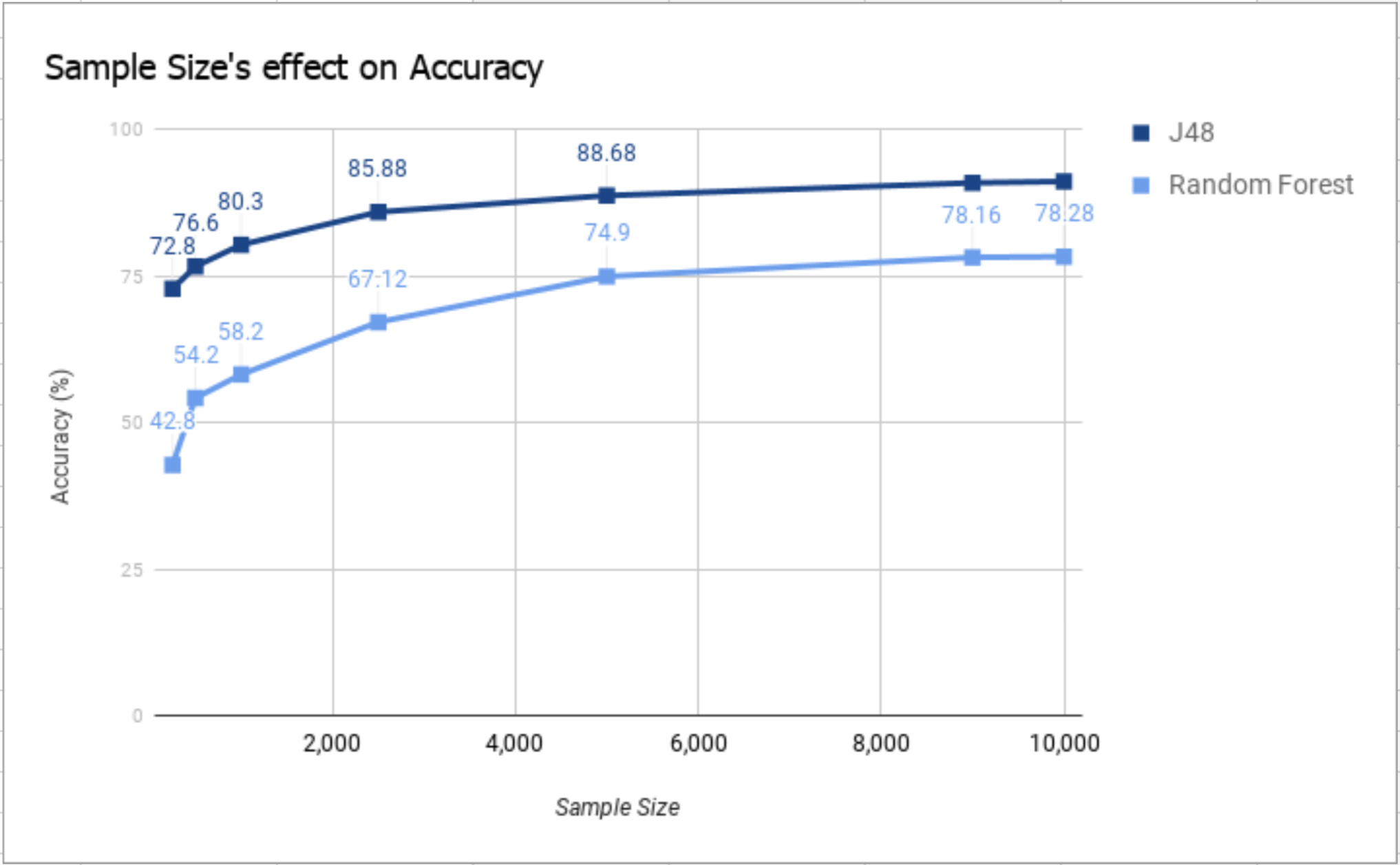
Our training set consists of 10,000 randomly-selected examples of taxi rides in New York in December 2017. Our testing set also consists of 10,000 randomly-selected taxi rides in New York, however the examples were selected from different months in 2017 such as September and July in order to better test the accuracy of our classifier. We had experimented with different sizes for the datasets, but ultimately chose a size of 10,000 examples. Our results from Figure 1 showed us that increasing the size of the dataset would not increase the accuracy, but decreasing the size would decrease the accuracy.
Before training, we changed the raw dataset to suit our needs. We added four additional attributes that were not a part of the raw dataset. Firstly, we used the pickup date of each example to find the day of the week that the ride took place. We represented day of the week as a number between 1-7, where 1 refers to Monday and 7 refers to Sunday. Additionally, we added an ‘IsWeekday?’ binary attribute, which is 1 when the ride took place on a weekday and 0 otherwise. This helped us account for the pricing and traffic differences that might take place on work days. Also, we rounded pickup time to the nearest hour to account for traffic patterns throughout the day. Lastly, we used the pickup and dropoff times and dates to calculate the durations of the rides.
We also rounded the fares to the nearest five dollars in our training set, so that our model’s output is nominal. We assume that our model will not need to predict fares outside of the range of fares in our 10,000 examples.
Our predictor only predicts the fare subtotal excluding fees and taxes, even though the raw dataset included it. This is because we assume that all additional fees and taxes are not as relevant to our goal of predicting fares based on all of our other inputs.
In summary, our final list of input attributes to our model are:
- Vendor ID (nominal)
- Day of Week (nominal)
- IsWeekday? (binary)
- Hour of Day (nominal)
- Duration (numeric)
- Passenger Count (nominal)
- Trip Distance (numeric)
- RatecodeID (nominal)
- Pick-up location ID (nominal)
- Drop-off location ID (nominal)
Our final output attribute is the fare rounded to the nearest five dollars.
Algorithm
We chose the decision tree algorithm because we surmised that the fare of the trip depended more heavily on particular attributes such as the duration of the trip. We ran our datasets through J48 and Random Forest classifiers. We also tested methods that were not decision trees such as Naive Bayes, ZeroR, and Nearest Neighbor. These methods did not perform as well as decision trees due to the nature of our dataset. Instead of using cross-validation, we chose to use a supplied test set to reduce the chance of overfitting.
See Table 1 for details.
Analysis
Based on our results from testing different classifiers, we can conclude that the best classifier for our dataset is a decision tree (J48 in Weka). With this classifier, we were able to obtain an accuracy of 91.09% using the testing set, compared to the other methods which all produced a lower accuracy. We found the duration and trip distance were the most informative attributes, followed by day of the week. This was supported by the fact that the decision tree splits on these attributes first. Also, when we take out these attributes from the dataset, the accuracy plummets. Without preprocessing the dataset, the accuracy for the J48 decision tree was 69.34%. This shows that each of the added attributes added value to the classifier and increased its accuracy. Finally, the accuracy of the classifier increases logarithmically in proportion to the amount of data points supplied in the dataset as shown in Figure 1.
Future Plans
While we managed to achieve a respectable accuracy using decision trees, there are many other steps we could take in the future to solidify our findings. Although we used pick-up location and drop-off location as part of our attributes, we did not have a definite understanding of New York’s zones and thus could not estimate traffic activity as an attribute. Additionally, we only procured data from New York in 2017, so we could try to test the same methods on data from different years or even cities to see exactly what factors affect the result the most. These steps could further increase the accuracy and expand the diversity of our examples.
Credits
- Jonathan Chan: Pre-processed data, tested data, contributed to final report, created website
- Ashu Gupta: Pre-processed data, tested data, contributed to final report
- Brian Liang: Pre-processed data, tested data, contributed to final report
- Kevin Mui: Pre-processed data, tested data, contributed to final report
Appendix
Table 1
Various method accuracies for 10,000 data points\ Demonstrates which classifier is the most accurate
| No. of data points | Classifier | Accuracy |
|---|---|---|
| 10,000 | J48 | 91.09% |
| 10,000 | Random Forest | 78.28% |
| 10,000 | Naive Bayes | 62.89% |
| 10,000 | Nearest Neighbor | 60.01% |
| 10,000 | ZeroR | 33.36% |
Figure 1
Sample Size’s effect on Accuracy\ Demonstrates sample size’s logarithmic relationship with accuracy